Friday, August 25, 2017

More HBase tuning


I've come across two HBase clusters where writes have been extremely fast and reads extremely slow. Note: these reads were not full scans (which would unsurprisingly be slow) but batched get() calls.

This post is about making HBase read things faster. "The rule of thumb is to have your hot data set in RAM. Does not fit? Increase RAM, increase # of servers." (from here).

How much data?

Check how big the HBase table is

hadoop fs -du -h  /hbase/data/default/ 

Compression

The more compressed your data, the more likely it is that it will all fit into RAM. Compressing data in the cache may increase CPU usages but reduce IO. You can check which native libraries Hadoop knows about with:

hadoop/bin/hadoop checknative -a

but note: "If the native libs are NOT present, you will see lots of Got brand-new compressor reports in your logs" (from here).

Wait for the cache to fill

It takes time for the cache to be populated. Run vmstat (on Unix-like OSs) and watch the number of blocks read (bi). It will be large to begin with (thousands or tens of thousands) then shrinks after the app has been running for a while, down to basically zero.

You can watch the progress in the region server's logs:

$ grep "BucketCacheStatsExecutor" hbase/logs/hbase-ubuntu-regionserver-ip-172-30-0-139.log
2017-08-23 09:15:28,192 INFO  [BucketCacheStatsExecutor] bucket.BucketCache: failedBlockAdditions=0, totalSize=5.86 GB, freeSize=4.28 GB, usedSize=1.58 GB, cacheSize=1.56 GB, accesses=49844, hits=2231, IOhitsPerSecond=7, IOTimePerHit=0.03, hitRatio=4.48%, cachingAccesses=49844, cachingHits=2231, cachingHitsRatio=4.48%, evictions=0, evicted=0, evictedPerRun=NaN
2017-08-23 09:20:28,192 INFO  [BucketCacheStatsExecutor] bucket.BucketCache: failedBlockAdditions=0, totalSize=5.86 GB, freeSize=837.15 MB, usedSize=5.04 GB, cacheSize=4.97 GB, accesses=150478, hits=33665, IOhitsPerSecond=104, IOTimePerHit=0.03, hitRatio=22.37%, cachingAccesses=150478, cachingHits=33665, cachingHitsRatio=22.37%, evictions=1, evicted=13644, evictedPerRun=13644.0
2017-08-23 09:25:28,192 INFO  [BucketCacheStatsExecutor] bucket.BucketCache: failedBlockAdditions=5, totalSize=5.86 GB, freeSize=552.66 MB, usedSize=5.32 GB, cacheSize=5.25 GB, accesses=299660, hits=95870, IOhitsPerSecond=207, IOTimePerHit=0.03, hitRatio=31.99%, cachingAccesses=299660, cachingHits=95870, cachingHitsRatio=31.99%, evictions=7, evicted=95977, evictedPerRun=13711.0

Types of caches

There are two types of caches: memcache and blockcache. The memcache is write-through cache. the blockcache is for read-only access.

You may want "to reduce the block size of the data stored in disk. Why? When a row is requested by client, the block corresponding to where the row is stored on disk (store file) is read into memory (cache) before sending it back the requested data to the client. So by decreasing the block size more relevant data can be stored in cache which can improve read performance." (from here).

Types of Blocks

From here: "HBase blocks and HDFS blocks are different things:

  • HBase blocks are the unit of indexing (as well as caching and compression) in HBase and allow for fast random access. 
  • HDFS blocks are the unit of the filesystem distribution and data locality"
Types of sizes

From here:

"Generally there are 2 sizes involved:

1. HBase Filesize
2. HBase Blocksize

#1 sets the maximum size of a region before it is split. Default used to be 512mb, it's now 1g (but usually it should be even larger)

#2 is the size of the blocks inside the HFiles. Smaller blocks mean better random access, but larger block indexes. I would only increase that if you have large cells."

Heap or off-Heap?

Making the cache off-heap really improved matters for me:

"When bucket cache is enabled in HBase, it will act as L2 (level 2 similar to processor cache hierarchy) cache and the default block cache will act as L1 cache. What that means is data need to be copied from L2 cache into L1 cache for HBase to service the query request. So on a read request when bucket cache is enabled, data block will be copied from disk onto bucket cache and then onto the block cache before served to the client making the request. On further reads of the same data, it will either be served directly from block cache or copied from bucket cache into block cache before serving the client request avoiding disk reads. So if there is a 10 node cluster with 128 GB of RAM each, it is possible to have almost 1 TB of data stored in HBase cache with bucket cache enabled and not get impacted by JVM GC which is not the case using just the default block cache." (from here).

So, trying assign more heap memory seems like a fool's errand. That will just cause a lot of GC. Instead, use off-heap memory.

Convolution


I was wondering if convolutional neural network had anything to do with convolution in mathematics. They do. But just as an introduction, here's what convolution in maths is all about.

Laplace transforms

These are useful in solving differential equations. Boaz defines them as:

L(f) = ∫f(t) e-pt dt = F(p)

If you use the key f(t), you can lookup the solution. For instance, if

f(t) =  e-at

then

F(t) = 1/(a + p)

You can work this out by simple integration, look it up in a table like this:
or use software like Sympy:

from sympy.abc import t, s
from sympy import *
import sympy

a = symbols('a', positive=True)
p = symbols('p')
print laplace_transform(sympy.exp(-a * t), t, p) 

which prints out:

(1/(a + p), 0, True)

Where this gets interesting is when we get recursive. Let f(t) = y and for brevity let y' = dy/dt etc. Let's plug this into the definition of a Laplace transformation at the top of the page:

L(y')y' e-pt dt

by a standard integration by parts (that says ∫u dv = uv - ∫v du) then with u=e-pt and dv=dy:

L(y') = y' e-pt dt = e-pt dy = e-pt y|0 - (-p)y e-pt dt
     = -y(0) + pL(y)

There was no particular reason to chose f(t) = y. In fact, let's chose f(t) = y' and do the same all over again. We get:

L(y'')  = -y'(0) + pL(y')

Taking these two equations, we can cancel out L(y') giving us:

L(y'')  = pL(y) - py(0) - y'(0)

and so on for any number of derivatives of y. We have our table of equations for L(y) so we only need plug that in.

Convolution

Now, as an example, take the equation:

A y''(t) + B y'(t) + C y(t) = f(t) where y(0) = y'(0) = 0

which is a typical physics equation (where a particle is at rest and the force applied to it start at at t=0). YMMV.

then applying the Laplace transform to all terms:

p2 L(y) + B p L (y) + C L(y) = L(f)

Re-arranging:

L(y) =      L(f)        =      L(f)
      (p+ B p + C)     A(p + a)(p + b) 

where a and b are chosen to make the constants B and C disappear.

But, as it happens, this factor is also a Laplace transform. From Boaz' table:

Let's call it T(p).

So, now we have:

L(y) = T(p) L(f)

and we can conclude that y "is the inverse transform of two functions whose inverse we know".

Ok, that's an example. Let's see the general case. Let G(p) and H(p) be transforms of g(t) and h(t) respectively. Then:

G(p) H(p) = g(σ) e-pσ dσ h(τ) e-pτ 

from the definition of a Laplace transformation (where we are using σ and τ to avoid confusion with a duplicated t).

Let's do another change of variables and have σ=t-τ for fixed τ which means that dσ=dt but the limits slightly change. So:

G(p) H(p) = τg(t-τ) e-p(t-τ)dt h(τ) e-pτ 
          = t=τ τ=0 e-pt g(t-τ) h(τ) dτ dt

Since τ ranges from 0 to ∞ and t from 0 to τ, the area we integrate over is the same as if t ranges from 0 to ∞ and τ from 0 to t. Therefore:

G(p) H(p) = L (t0 g(t-τh(τ) dτ ) = L ( g * h )

Note that τ introduces a sliding window that will be used in convolutional neural nets (part 2).


Wednesday, August 9, 2017

3D Plots


I'm creating a Spark linear algebra library but wanted to plot a few graphs to get an idea of what's going on. These are the tools I tried.

Sympy

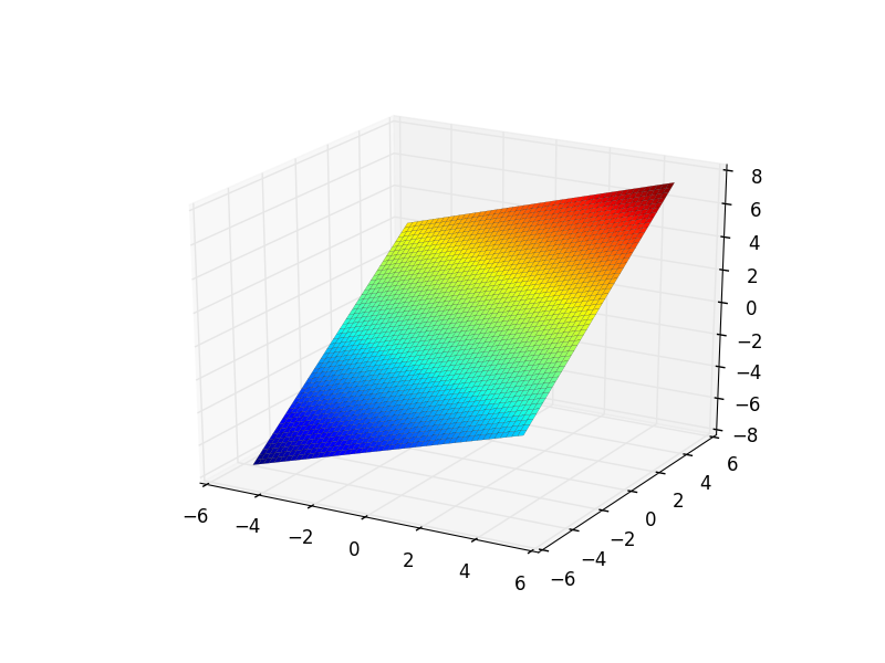
Sympy looked good as it allowed implicit functions. For instance, you can write:

from sympy import symbols
from sympy.plotting import plot3d

x, y = symbols('x y')

p = plot3d((x/2) + y, (x, -5, 5), (y, -5, 5))

and get the plane that represents z = (x/2) + y.

The problem was that "SymPy uses Matplotlib  behind the scenes to draw the graphs" [1] and Matplotlib has some issues in the z-order while rendering.

So, although SymPy gives you a lot more than just plotting, I moved on to...

Mayavi

... which renders things beautifully.

Until I tried to do something clever.

First, I had to update pip. Then, with, I tried:

from mayavi import mlab
.
.
mlab.options.backend = 'envisage'

which gave me:

ImportError: No module named envisage.ui.workbench.api

And after some googling, it looked like I needed to mess around with all sorts of libraries so I was a coward and gave up quickly.

Jzy3d

It turns out that there is a perfectly good Java library called Jzy3d which is quite mature.

Given:

v1 = [8, -2, 2]
v2 = [4,  2, 4]

I wanted to plot these vectors, the surface on which they lie and the shortest distance between this plane and [5, -5, 2] (this exercise can be found in Philip Klein's excellent "Coding the Matrix").

First, I had to convert this information to something Jzy3d can handle - which looks like this:

        Mapper plane = new Mapper() {
            @Override
            public double f(double x, double y) {
                return (x + (2 * y)) / 2;
            }
        };

that is, we first need to turn these vectors into an implicit function. Well, any point (x, y, z) on the plane can be described as s v1 + t v2 where s and t are any real numbers. Turning this information into parametric equations is easy:

x = 8s  + 4t
y = -2s + 2t
z = 2s  + 4t

and solving these simultaneous equations gives us the implicit function:

x + 2y - 2z = 0

or

z = (x + (2 * y)) / 2

which is the equation we find in our Java code above.

Finding the normal to an implicit function is simply the coefficients, that is [1, 2, -2]. At the point the normal meets [5, -5, 2] (which we'll call b) is the point where u b =s v1 + t v2. Once again, convert to parametric equations and then solve the simultaneous equations and you'll find t=-0.5 and s=1. This will give the point [6, -3, 0] and Jzy3d renders it like this:


where the red line is the normal, the green line is the point and the blue line is the closest point on the surface.

The rendering can be a bit jagged and I need to look at adding arrows to the vectors but so far, this seems to be the easiest plotting library to use.

[1] Doing Math with Python (No Starch Press)